History of eBPF

Origins of BPF (Berkeley Packet Filter)

The origins of eBPF (extended Berkeley Packet Filter) trace back to its predecessor, the Berkeley Packet Filter (BPF). BPF was first introduced in 1992 by Steven McCanne and Van Jacobson at the Lawrence Berkeley Laboratory. It was designed to provide a high-performance, user-programmable packet filtering mechanism for network monitoring tools, particularly for capturing packets in real-time.

Prior to BPF, packet capturing was inefficient due to the need for constant context switching between the kernel and user space. The kernel would pass every network packet to user space, where filtering decisions were made. This approach led to significant overhead. BPF addressed this problem by enabling the execution of filtering programs directly within the kernel, allowing only relevant packets to be passed to user space. This dramatically improved performance and efficiency.

Classic BPF and Its Limitations

Classic BPF, often referred to as cBPF worked by allowing users to write simple programs to filter network traffic based on specific patterns. These programs were expressed as sequences of low-level instructions that the BPF virtual machine (VM) running in the kernel could interpret and execute. The most notable tool that leveraged cBPF was tcpdump, which allowed network administrators to capture and analyze network packets effectively.

Despite its efficiency, cBPF had several limitations:

1. Limited Instruction Set: The instruction set of classic BPF was restricted to basic filtering operations, making it unsuitable for more complex use cases.
2. Single-Purpose: cBPF was designed primarily for packet filtering. It lacked the flexibility to perform tasks beyond network monitoring.
3. 32-bit Architecture: Classic BPF programs operated on 32-bit registers, which limited performance and data processing capabilities.
4. Lack of Extensibility: There was no straightforward way to extend the functionality of cBPF beyond packet filtering.

Integration of BPF into the Linux Kernel

BPF was first integrated into the Linux kernel in 1997, starting from version 2.1. This integration allowed kernel-level packet filtering for tools like tcpdump and iptables. Over time, the BPF VM became a reliable mechanism for filtering network traffic efficiently within the kernel space.

However, as system and network performance demands grew, the limitations of classic BPF became more clear. The need for a more powerful, flexible, and extensible version of BPF led to the development of eBPF.

Introduction and Evolution of eBPF (2014-Present)

In 2014, the Linux kernel version 3.18 introduced “extended BPF” (eBPF). eBPF was a significant enhancement over classic BPF, providing a modern, flexible, and powerful framework for executing user-defined programs within the kernel. The key improvements introduced by eBPF include:

1. 64-bit Registers: eBPF uses a 64-bit architecture, which improves performance and data-handling capabilities.
2. General-Purpose: eBPF is no longer limited to packet filtering; it can be used for various tasks, including tracing, performance monitoring, security enforcement, and more.
3. Extensible and Safe: eBPF programs are verified by an in-kernel verifier to ensure safety, preventing programs from crashing the kernel or causing security vulnerabilities.
4. Just-In-Time (JIT) Compilation: eBPF programs can be compiled into native machine code at runtime, which significantly improves execution speed.
5. Maps and Helpers: eBPF supports maps (key-value storage) and helper functions that provide interaction between eBPF programs and the kernel.

Since its introduction, eBPF has evolved rapidly, with continuous enhancements to its feature set and performance. Projects like bcc (BPF Compiler Collection), bpftool, and libbpf have made writing and deploying eBPF programs more accessible. eBPF is now used extensively for networking, observability, and security tasks in major projects like Cilium, Falco, and the Kubernetes ecosystem.

Naming Confusion

The terminology surrounding BPF and eBPF often leads to confusion due to the historical evolution of the technology. Originally, BPF referred exclusively to the Berkeley Packet Filter designed for packet capture. However, with the introduction of eBPF in 2014, the technology evolved far beyond its initial purpose, supporting tasks like tracing, performance monitoring, and security.

Despite these advancements, many tools and kernel APIs continue to use the term “BPF” even when referring to eBPF functionality. For example, commands like bpftool and the bpf() system call refer to eBPF features while retaining the older name. This overlap in terminology can cause misunderstandings, especially for newcomers who may not be aware of the differences between classic BPF and modern eBPF.

To avoid confusion, it’s helpful to use “BPF” when referring to the original packet-filtering technology and “eBPF” when discussing the extended capabilities introduced in the modern framework. This distinction clarifies communication and ensures a better understanding of the technology’s capabilities in the Linux ecosystem.

Example Using tcpdump

To illustrate classic BPF in action, consider a simple tcpdump command that captures only TCP traffic on port 80 (HTTP):

tcpdump -i eth0 'ip and tcp port 80'

This command filters packets to capture only those that are TCP-based and are using port 80. The underlying BPF bytecode generated by this command can be viewed using the -d flag:

tcpdump -i eth0 -d 'ip and tcp port 80 tcp port 80'

The output might look like this:

(000) ldh      [12]
(001) jeq      #0x800           jt 2    jf 12
(002) ldb      [23]
(003) jeq      #0x6             jt 4    jf 12
(004) ldh      [20]
(005) jset     #0x1fff          jt 12   jf 6
(006) ldxb     4*([14]&0xf)
(007) ldh      [x + 14]
(008) jeq      #0x50            jt 11   jf 9
(009) ldh      [x + 16]
(010) jeq      #0x50            jt 11   jf 12
(011) ret      #262144
(012) ret      #0

Explanation of the Generated BPF Bytecode

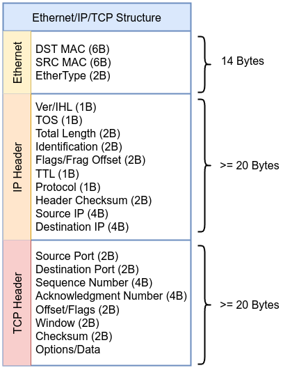
Before diving into the example, take a moment to review the following diagram of the Ethernet, IP, and TCP headers. This will help you visualize how the packet is structured, making it easier to follow along with each step in the BPF bytecode. Keep this scheme in mind as we go through the example to understand how each instruction maps to specific parts of the packet.

Here’s the breakdown of each instruction, including the relevant source code location and snippets from the Linux kernel where these actions are defined or represented.

1. Instruction 000 ldh [12]: Load the 16-bit EtherType field at offset 12 in the packet as described in the kernel source code include/uapi/linux/if_ether.h

   #define ETH_HLEN 14          /* Total Ethernet header length */
   #define ETH_P_IP 0x0800      /* IPv4 EtherType */
   

2. Instruction 001 jeq #0x800 jt 2 jf 12: If the EtherType is 0x800 (IPv4), jump to instruction 2; otherwise, jump to instruction 12.

3. Instruction 002 ldb [23]: Load the 8-bit protocol field at offset 23 in the IP header.

4. Instruction 003 jeq #0x6 jt 4 jf 12: If the protocol is 6 (TCP), jump to instruction 4; otherwise, jump to instruction 12 as described in the kernel source code include/uapi/linux/in.h

   #define IPPROTO_TCP 6        /* Transmission Control Protocol */
   

5. Instruction 004: ldh [20]: Load the 16-bit TCP source port at offset 20.

6. Instruction 005: jset #0x1fff jt 12 jf 6: Check if the lower 13 bits of the TCP header are non-zero; if true, jump to instruction 12; otherwise, jump to instruction 6.

7. Instruction 006: ldxb 4*([14]&0xf): Load the value in the TCP header, adjusting by scaling based on the value in the IP header.

8. Instruction 007: ldh [x + 14]: Load the TCP destination port, located at offset 14 from the start of the packet.

9. Instruction 008: jeq #0x50 jt 11 jf 9: If the destination port is 80 (0x50 in hexadecimal), jump to instruction 11; otherwise, jump to instruction 9.

10. Instruction 009: ldh [x + 16]: Load the TCP source port, located at offset 16 from the start of the packet.

11. Instruction 010: jeq #0x50 jt 11 jf 12: If the source port is 80 (0x50), jump to instruction 11; otherwise, jump to instruction 12.

12. Instruction 011: ret #262144: If all conditions match, capture the packet (return the packet length).

13. Instruction 012: ret #0: If the conditions do not match, drop the packet.

These instructions illustrate a classic BPF packet filter that matches IPv4 and TCP traffic on port 80 (HTTP). The constants and structures provided are standard definitions in the Linux kernel. This bytecode demonstrates how classic BPF allows efficient filtering by executing a series of low-level instructions directly in the kernel.

Let’s explore the differences between classic BPF and eBPF to better understand the enhanced capabilities of eBPF.

Classic BPF vs. eBPF

As mentioned, Berkeley Packet Filter (BPF) was originally developed to filter network packets efficiently. It enabled in-kernel filtering of packets based on simple criteria. However, as the need for more versatile and performant filtering and monitoring grew, extended BPF (eBPF) emerged as a powerful evolution. eBPF transforms BPF into a general-purpose execution engine within the kernel, providing significantly more flexibility and efficiency.

The following 6 points explores the key differences between eBPF and classic BPF, based on Kernel Documentation https://docs.kernel.org/bpf/classic_vs_extended.html.

Use Cases

Classic BPF is primarily used for packet filtering. Its primary use case is in network monitoring tools like tcpdump, where it allows users to specify packet filtering rules directly within the kernel.

eBPF, however, has vastly expanded use cases. eBPF is used in:

• System monitoring: Collecting detailed information on kernel events such as system calls, file access, and network traffic.
• Performance profiling: Monitoring the performance of different parts of the kernel, applications, or system calls in real-time.
• Security: Tools like seccomp (Secure Computing Mode) use eBPF to filter system calls, enforcing security policies directly at the kernel level.
• Tracing: Tracing the execution of kernel functions and user programs, providing insights into system behavior.

Instruction Set and Operations

Classic BPF has a very limited instruction set, primarily designed for basic operations like loading data, performing simple arithmetic, jumping, and returning values.

eBPF, in contrast, expands the instruction set significantly. It introduces new operations like:

• BPF_MOV for moving data between registers,
• BPF_ARSH for arithmetic right shift with sign extension,
• BPF_CALL for calling helper functions (which will be explained in more details later).

Additionally, eBPF supports 64-bit operations (via BPF_ALU64) and atomic operations like BPF_XADD, enabling more sophisticated processing directly in the kernel.

Registers and Data Handling

Classic BPF only has two registers (A and X), with limited memory and stack space. The operations on data are simple and restricted to 32-bit width, and these registers are manipulated with specific instructions that limit flexibility.

eBPF greatly improves on this by expanding the number of registers from 2 to 10. eBPF’s calling conventions are designed for high efficiency, utilizing registers (R1-R5) to pass arguments directly into the kernel functions. After the function call, registers R1-R5 are reset, and R0 holds the return value.This allows for more complex operations and handling of more data. Registers in eBPF are also 64-bit wide, which enables direct mapping to hardware registers on modern 64-bit processors. This wider register set and the introduction of a read-only frame pointer (R10) allow eBPF to handle more complex operations like function calls with multiple arguments and results.

JIT Compilation and Performance

Classic BPF is interpreted by the kernel, This means the kernel would read and execute each instruction one by one which adds overhead to the execution of each instruction. This can be a limiting factor when performing more complex operations or filtering on high-throughput systems.

eBPF is designed with Just-In-Time (JIT) compilation in mind, meaning that eBPF programs can be translated into optimized native machine code at runtime. The JIT compiler can convert eBPF bytecode to highly efficient machine instructions, reducing the overhead significantly. This allows eBPF programs to perform at speeds comparable to native code execution, even for complex tasks like system call filtering and network traffic analysis.

Safety and Verifier

Classic BPF uses a simple verifier that checks for program safety by ensuring there are no errors like out-of-bounds memory access.

eBPF, on the other hand, includes a more sophisticated verifier that ensures the program complies to a set of strict rules before execution. The verifier checks for issues like:

• Accessing invalid memory regions,
• Ensuring correct pointer arithmetic,
• Verifying that all function calls are made with valid arguments.

This makes eBPF programs much safer, even when they are running with elevated privileges or performing sensitive tasks in the kernel.

Program Size and Restrictions

Classic BPF: The original BPF format had a program size limit of 4096 instructions, and programs had to be very efficient to avoid exceeding this limit. The limited number of registers and operations meant that programs were usually simple and short.

eBPF: While eBPF still retains a 4096 instruction limit for kernels before 5.2 and one million instructions for kernel starting from 5.2, its expanded instruction set and register size allow for significantly more complex programs. Additionally, the eBPF verifier ensures that programs are safe, loop-free, and deterministic. Furthermore, there are restrictions on the number of arguments that can be passed to kernel functions (currently up to five), although these can be relaxed in future versions of eBPF. Tail calls also allow chaining multiple eBPF programs together, effectively extending the overall execution beyond the single-program instruction limit.

Now, let’s dive into real-world examples to see how eBPF is applied in action and understand its practical benefits.